Flow Dynamics – Chapter 3

Explore the role of resonance as the heartbeat of the RLFlow Model.

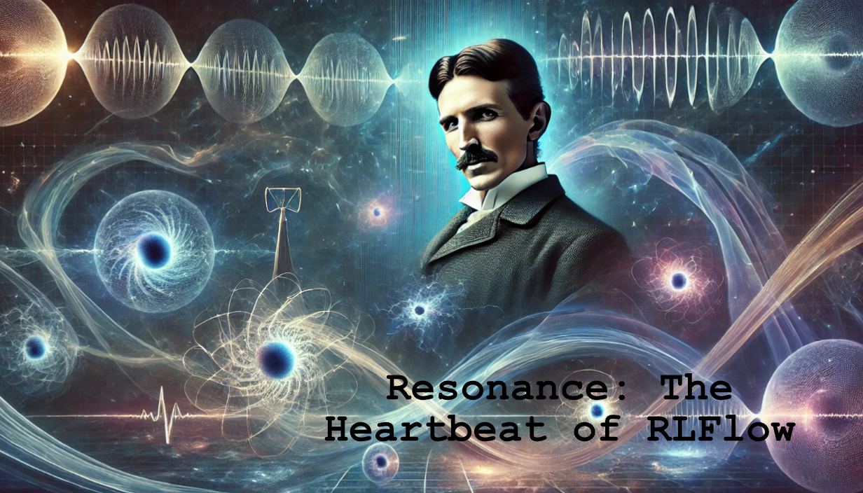
Resonance: The Heartbeat of RLFlow

In the RLFlow model, resonance is the heartbeat of how flows interact, shaping the very fabric of reality. Imagine resonance as the rhythm at which different flows align, amplify, or even cancel each other out. To truly understand RLFlow, we need to dive into the concept of resonance and how it describes the dynamics within the flowfield, which helps explain everything from particles to cosmic forces.

The Resonance Factor

To describe resonance mathematically, we use an equation called the Resonance Factor:

Resonance Factor = (Flow Changes) + (Flow Fluctuation Strength) × sin((Oscillation Frequency × Time) + Phase Shift)

This equation is fundamental to understanding how flows behave in RLFlow. It tells us that the behavior of any flow is influenced by how the flow changes over time, as well as by natural fluctuations and oscillations within the flow. Let’s break down what each component of the Resonance Factor means.

Breaking Down Flow Changes

The first part of the equation, Flow Changes, represents the dynamics within the flow that can vary over time. Specifically:

Flow Changes = (Velocity Change) + (Pressure Change) + (External Forces)

• Velocity Change: This term describes how the speed of the flow is changing over time and across different locations. Think of how a river might flow faster in some spots and slower in others—this variability is what we call velocity change.
• Pressure Change: This refers to how the pressure within the flow changes in response to its environment. Areas of higher or lower pressure influence how the flow behaves—much like how water pressure influences whether a stream rushes quickly or meanders slowly.
• External Forces: These are forces that come from outside the flow, like gravity or wind, that act upon it. They shape and redirect the flow, often creating new patterns or changing existing ones.

Flow Changes are all about the internal and external influences that alter the flow’s state, giving it variability and complexity.

Flow Fluctuation and Oscillation

The second part of the Resonance Factor equation involves Flow Fluctuation Strength and oscillations:

• Flow Fluctuation Strength (η): This represents the amplitude, or the strength, of natural fluctuations in the flow. No flow is ever perfectly steady—even calm rivers have tiny ripples and movements. The amplitude tells us how strong these fluctuations are.
• Oscillation Frequency (ω): This is how often the flow fluctuates over time—in other words, the rhythm of the flow. Is it slow and steady like a gentle breeze, or fast and erratic like turbulent rapids?
• Phase Shift (δ): This represents how in-sync the oscillations are with other elements in the flow. It tells us if the flow is starting its oscillations a little earlier or later than another part of the system.

Together, these components describe how a flow naturally fluctuates over time, creating patterns that can be stable or chaotic depending on how the different elements come together.

Resonance and Flow Potential in the RLFlow Framework

The Resonance Factor is a critical component of the RLFlow model, capturing the behavior of flows and helping explain how various physical phenomena emerge from the interactions of these flows. Resonance provides a unifying concept that reveals how seemingly disparate entities, such as particles and forces, are interconnected through the dynamics of flow.

The Resonance Equation Restated:

R(x, t) = f(∇u(x, t), ∇p(x, t), f_ext(x, t)) + η · sin(ωt + δ)

Key Components Recap:

R(x, t): Represents the intensity and stability of the flow at any given point, essentially describing how "strong" or "resonant" the flow is.

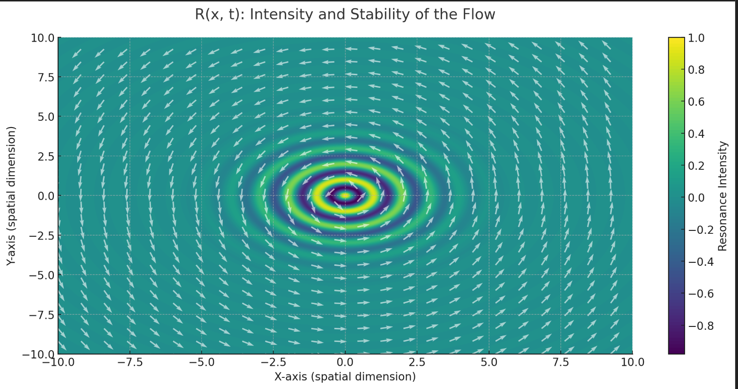
Here is the visual representation for R(x,t), showcasing the intensity and stability of the flow at given points. The resonance intensity is depicted as a Gaussian field modulated with oscillatory behavior, while the flow vectors illustrate the dynamic nature of the flowfield.

Flow Changes f(∇u, ∇p, f_ext):

• ∇u(x, t): Velocity gradient—describes changes in the flow's speed, showing how quickly it varies across space.
• ∇p(x, t): Pressure gradient—indicates changes in the pressure across the flowfield, important for defining the local behavior.
• f_ext(x, t): External forces—such as gravity, electromagnetic effects, or other influences that alter the flow.

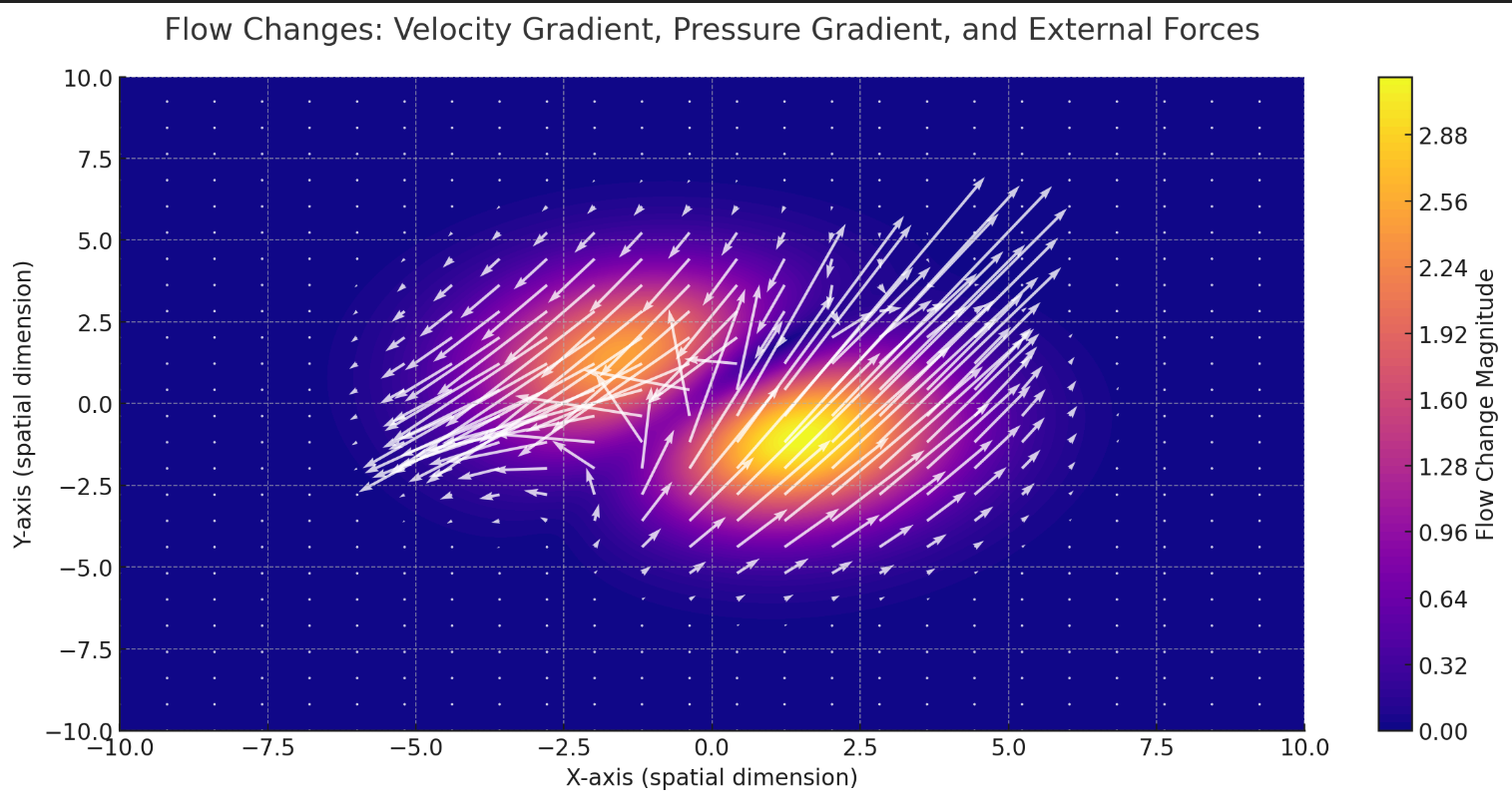
This visualization represents Flow Changes as the combination of velocity gradients (∇u), pressure gradients (∇p), and external forces (f_ext). The color map indicates the magnitude of the flow changes, while the vectors overlaying the plot illustrate the dynamic interplay of these components.

The first part of the equation, f(∇u(x, t), ∇p(x, t), f_ext(x, t)), sets the underlying “shape” or steady pattern of the flow’s resonance. This baseline depends on how the flow’s velocity, pressure, and external forces change over space and time. Without the sine term, the resonance would describe a certain intensity that could vary smoothly but wouldn’t necessarily have a regular, rhythmic fluctuation.

Oscillatory Term (η · sin(ωt + δ)):

• η: Amplitude of natural flow fluctuations.
• ω: Frequency of oscillation, dictating how often the flow oscillates.
• δ: Phase shift, accounting for timing differences in these oscillations.

The second term, η · sin(ωt + δ), adds a time-dependent oscillation to that baseline:

• sin(ωt + δ): The sine function ensures that the flow intensity doesn’t just stay at a single level; it now cycles up and down over time.
• η (Amplitude): This factor scales how strong those oscillations are. If η is large, the resonance will swing widely above and below the baseline set by f(…). A small η means only gentle ripples or minor fluctuations.
• ω (Frequency): The frequency, ω, tells you how often the resonance completes one cycle (from peak to trough and back to peak) in a given time frame. Higher ω means the oscillations happen more rapidly, lower ω means they’re more gradual.
• δ (Phase Shift): The phase shift, δ, changes where in its cycle the sine wave starts at t=0. Rather than starting at zero, it could begin at a peak, a trough, or anywhere in between. This affects how different regions or factors in the flow interact with one another over time.

Let’s talk more about the Sine Function

Basic Definition

The sine function maps an angle (θ) to a value between -1 and 1.

• When θ = 0°, sin(0°) = 0.
• When θ = 90°, sin(90°) = 1.
• When θ = 180°, sin(180°) = 0.
• When θ = 270°, sin(270°) = -1.
• When θ = 360°, sin(360°) = 0 again, completing one full cycle.

Periodic and Cyclical Nature

One of the most important features of the sine function is that it’s periodic. After a certain interval (360° or 2π radians), sin(θ) repeats its pattern. This makes it perfect for modeling anything that repeats in a regular cycle—such as sound waves, light waves, or the natural fluctuations of a flowfield.

Modeling Oscillations

Many real-world systems fluctuate or oscillate about an equilibrium point. Whether it’s a spring bouncing up and down, a pendulum swinging back and forth, or waves in water, these can often be described by sine (or related) functions. In the RLFlow model:

• The sine function represents how the intensity of a flow fluctuates over time.
• By adjusting parameters like frequency (how rapidly it oscillates) and phase (where in its cycle it starts), we can capture a wide range of behaviors.
• The amplitude (η) sets how “tall” the sine wave’s peaks and troughs are, controlling the strength of the flow’s oscillations.

Phase and Frequency in Context

• Frequency (ω): If we consider sin(ωt), the factor ω controls how fast the oscillation occurs. A larger ω means the sine wave repeats more times per unit of time.
• Phase Shift (δ): If we consider sin(ωt + δ), the δ term shifts where in its cycle the sine function starts. Instead of starting at sin(0) = 0, it might begin at a peak or a trough, changing how multiple oscillations interact.

Resulting Behavior:

• During certain times, the sine term may push the total resonance higher, creating conditions more favorable for stable patterns.
• At other times, the sine term lowers the resonance, introducing conditions that are more chaotic or less stable.

Physical Interpretation:

In a physical sense, this means that real flow systems aren’t static. They naturally exhibit cycles of intensity and stability, much like ocean waves or the vibrations of a string. The sine function is the mathematical tool that captures this cyclical nature. It makes the equation reflect reality more closely, where nothing is perfectly still and everything is in a state of continuous fluctuation.

In short, the sine function in this equation injects periodic, time-dependent variations into the resonance factor, making the system dynamic, ever-changing, and more true to the complexities of real-world flows.

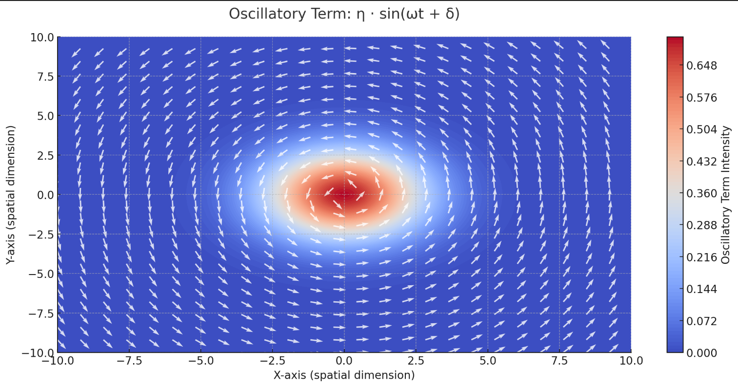
This visualization represents the Oscillatory Term η⋅sin(ωt+δ), showing the oscillations across the flowfield. The color map highlights the intensity of the oscillatory fluctuations, while the vector field illustrates the directional ripples caused by these oscillations.

Understanding Resonance: The River Analogy

To understand the Resonance Factor, it helps to visualize a river:

Flow Velocity (∇u):

Imagine sections of the river where water moves smoothly, and others where it forms rapids. The changes in velocity across these sections represent the velocity gradient.

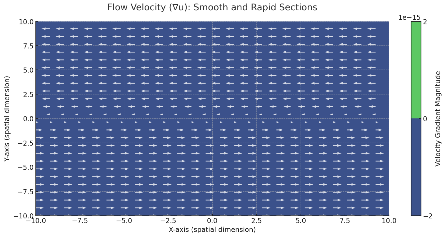
This visualization depicts Flow Velocity (∇u), illustrating sections of smooth flow and areas of rapid changes, akin to a river's dynamics. The color map represents the magnitude of velocity gradients, while the overlaid vectors show the direction and speed of the flow.

Pressure Gradient (∇p):

The water pushes more intensely in certain areas, leading to either gentle currents or powerful surges, depending on the local pressure gradient.

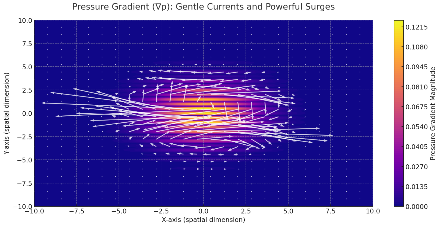
This visualization illustrates the Pressure Gradient (∇p), showing areas of gentle currents and powerful surges. The color map highlights the magnitude of pressure changes across the flowfield, while the vectors represent the direction of pressure-driven forces.

External Forces (f_ext):

Imagine wind blowing across the river, or a stone thrown into the water. These are external forces that modify the natural flow, creating disturbances and altering its behavior.

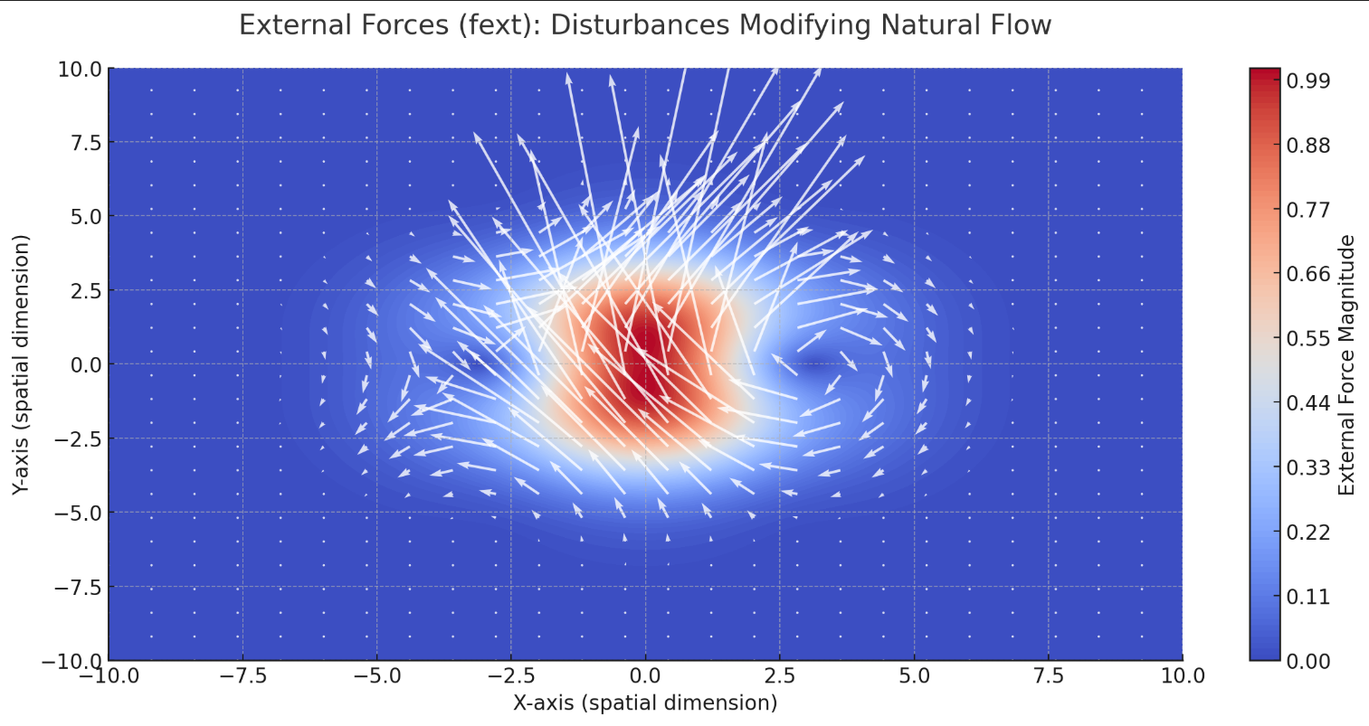
This visualization captures External Forces (f_ext), illustrating how disturbances, such as wind or obstacles, modify the natural flow. The color map shows the intensity of these forces, while the vectors represent their direction and impact on the flowfield.

Oscillations (η · sin(ωt + δ)):

Just as ripples form on the surface of a river, flows naturally experience oscillations. These ripples depend on local disturbances, and their intensity and timing are represented by the amplitude, frequency, and phase of the oscillatory term.

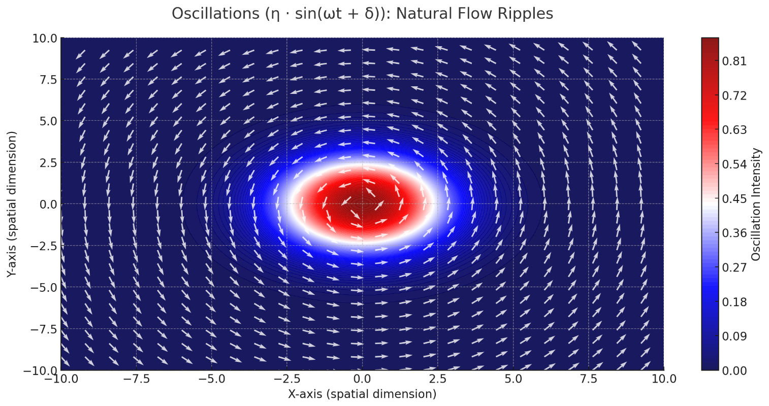
This visualization represents Oscillations (η⋅sin(ωt+δ)), illustrating the natural ripples and fluctuations within a flowfield. The color map highlights the intensity of the oscillations, while the vector overlay shows the directional disturbances caused by these oscillatory terms.

Resonance Intensity, Velocity Gradient, Pressure Gradient, External Forces, and Oscillatory Terms

(Resonance Intensity):

This is like a measure of how “lively” or “stable” the flow is at a particular location and time. High resonance means the flow pattern is strong and steady; low resonance means it’s weaker or more chaotic.

(Velocity Gradient):

Shows how the flow’s speed changes over space. If one spot is fast and another nearby is slow, the difference in speeds (the gradient) tells you the flow isn’t uniform.

Imagine watching a river: the water near the center moves faster than the water at the edges. That difference in speed is the velocity gradient.

(Pressure Gradient):

Shows how pressure changes from one point to another. Pressure differences can push the flow around.

Think of opening a door on a windy day: the difference in air pressure inside and outside can create a breeze that moves air through the doorway.

(External Forces):

Represents outside influences like gravity or electromagnetic fields acting on the flow.

Imagine tipping a container of water: gravity pulls the water downward, changing its flow pattern.

(Oscillatory Term):

On top of that baseline, the flow naturally “wiggles” or oscillates. This term represents that extra layer of fluctuation:

(Amplitude):

How big these oscillations are. Larger η means more pronounced waves or ripples.

Imagine gentle ripples on a pond versus big waves—the amplitude tells you how tall the waves get.

(Frequency):

How often these oscillations occur. Higher frequency means the flow pattern changes more rapidly over time.

A hummingbird’s wings flap at a higher frequency than a pigeon’s. Similarly, higher ω means more frequent “wiggles” in the flow.

(Phase Shift):

Where in its cycle the oscillation starts. It determines if the ripple begins at a peak, a trough, or somewhere in between.

Think of two people bouncing on a trampoline: if one starts just as the other reaches the top of a bounce, their “phases” are offset.

Putting It All Together:

The flow’s resonance, R(x,t), is shaped first by how speed and pressure change and what external forces are at play. This sets the main pattern of the flow—like deciding if a river runs smoothly or has lots of eddies.

Then, on top of this pattern, you add the natural “wiggles” or oscillations, which make the flow fluctuate rhythmically.

The result is a complete picture of the flow’s intensity and stability, capturing both steady influences (like pressure and gravity) and the lively, rhythmic fluctuations (like gentle waves) that give the flow its character.

The Broader Implications of Resonance in RLFlow

In the RLFlow model, resonance is the foundation that explains the behavior of physical systems at multiple levels. The resonance of a flow determines how it interacts with others, giving rise to phenomena we observe in classical and quantum physics.

1. Particles as Stable Resonances

• In the RLFlow model, particles are not static points but vortices of stable resonance. They are concentrated regions where the flow has formed a stable pattern, much like a whirlpool in a river.
• These stable flows, or vortices, are what we perceive as "particles," and their stability is directly related to the resonance factor. If the resonance of a flow is high and stable, it forms a particle-like structure, while lower or more dynamic resonance leads to more fluid, wave-like behaviors.

2. Forces as Flow Interactions

• Forces, such as gravity or electromagnetism, are emergent properties that result from the interaction of different flows. The strength and direction of these interactions are determined by how the resonance of two or more flows interacts.
• Instead of viewing forces as mysterious interactions mediated by discrete particles, RLFlow suggests they are the natural outcome of resonant flows influencing each other. Gravity, for instance, could be viewed as the effect of one massive flow bending and altering the resonance of nearby flows.

3. Energy as Intensity of Resonance

• Energy in the RLFlow model is related to the intensity of flow interactions and fluctuations. Just like the faster-moving parts of a river have more energy, regions of intense resonance represent areas of high energy.
• Kinetic energy can be seen as the movement and velocity of the flow, while potential energy is linked to the flow's configuration and its ability to influence other flows. The resonance factor captures this energy as it varies with time and position.

Connecting Resonance with Classical and Quantum Worlds

The resonance concept bridges the gap between classical mechanics, as laid out by Newton, and the more abstract quantum mechanics introduced by Schrödinger, Heisenberg, and others. Here are some key connections:

Resonance and Quantum Mechanics

• In the quantum world, particles like electrons and photons exhibit both wave-like and particle-like behaviors. The RLFlow model suggests that these behaviors are manifestations of the resonance of the flowfield.
• For example, an electron is not a discrete object but a resonant flow vortex whose stability changes depending on how it interacts with other flows or fields.
• The oscillatory term (η · sin(ωt + δ)) reflects the probabilistic nature of quantum particles. It helps explain phenomena like quantum superposition—the idea that particles can exist in multiple states at once, which in RLFlow is represented by the overlapping, resonating flows.

Heisenberg’s Uncertainty Principle Reimagined

• The uncertainty principle, which states that we cannot simultaneously know a particle's position and momentum with perfect precision, finds a natural explanation in RLFlow.
• The fluctuations in flow resonance, described by the oscillatory term, introduce an inherent unpredictability. These fluctuations mean that the flow is constantly shifting, making it impossible to measure certain properties without affecting others.

Metaphor: Flows as Dancers in a Cosmic Ballet

Think of flows as dancers in a ballet, moving across the stage (the flowfield):

• Each dancer represents a flow, and their movements are dictated by the resonance—some dancers move slowly and gracefully, while others move with intense speed and energy.
• The interaction between dancers—how they twist, turn, or respond to each other—represents the forces we perceive.
• The entire ballet is guided by the music, which represents the external forces (f_ext) and dictates the rhythm (ω) and intensity (η) of the performance.
• Sometimes, two dancers move in perfect harmony, their actions mirroring each other—this is reciprocal resonance. At other times, they move unpredictably, shifting suddenly, much like quantum particles.

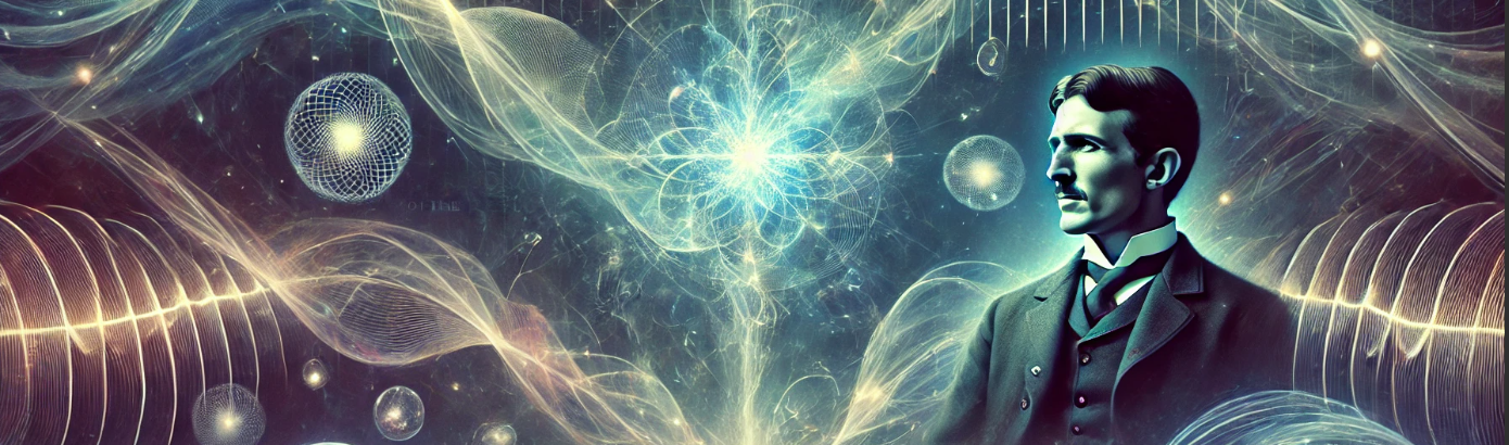
Resonance and the Vision of Nikola Tesla

To fully appreciate the depth of the Resonance Factor within the RLFlow model, it’s insightful to connect these ideas to the visionary work of Nikola Tesla. Tesla’s fascination with resonance, vibration, and the interconnectedness of energy and matter resonates profoundly with RLFlow’s principles. He once said, "If you want to find the secrets of the universe, think in terms of energy, frequency, and vibration." This statement forms a philosophical cornerstone for RLFlow and its resonance-based understanding of reality.

Tesla’s Vision of Energy, Frequency, and Vibration

• Tesla’s exploration of electromagnetic waves and his development of technologies like resonant transformers reflect his deep understanding of resonance. He knew that resonance could amplify energy, stabilize oscillations, and bring disparate elements into harmony.
• In RLFlow, resonance is the heartbeat of all flows—the underlying factor that connects energy, mass, and forces. Tesla envisioned a world where energy flowed freely, unobstructed, and harmoniously resonated across systems. RLFlow expands on this idea, suggesting that not only is energy interconnected, but that everything—from gravity to consciousness—is fundamentally about flow and resonance.

Resonance Unifying Natural Forces

The Resonance Factor provides a framework for unifying all the natural forces. Through resonance, it becomes clear that phenomena such as gravity, electromagnetism, and even quantum mechanics are not distinct entities but expressions of how different flows interact. Tesla’s belief in the unification of energy echoes through this model, where no phenomenon stands alone—all are interconnected parts of a great cosmic flow.

1. Gravity as Resonant Flow Curvature

• In RLFlow, gravity is no longer viewed as a force transmitted through space by particles like gravitons or through the warping of spacetime alone. Instead, gravity is the result of resonant flow curvature—a large flow (like a planet or star) creates a deep well in the flowfield, affecting the flows around it.
• Tesla was fascinated by the forces that shaped the universe, and he sought to understand how these forces could be tapped into. The RLFlow model aligns with his vision by showing that gravity itself can be understood and possibly manipulated through understanding resonance.

2. Electromagnetism and Flow Resonance

• Electromagnetic waves, as Tesla demonstrated, are oscillations of electric and magnetic fields. In RLFlow, these oscillations are better understood as resonances within the flowfield. The amplitude (η), frequency (ω), and phase shift (δ) components of the Resonance Factor help describe the behavior of electromagnetic flows.
• Tesla envisioned wireless power transmission, a dream where energy would flow freely, carried by resonant waves across vast distances. The RLFlow model offers the possibility of taking this dream even further—if resonance dictates the behavior of flows, it might be possible to manipulate not only electromagnetic energy but also gravity and quantum states through controlled resonance.

3. Quantum Fluctuations as Resonant Oscillations

• At the quantum scale, RLFlow’s Resonance Factor offers a fresh perspective on quantum behavior. Tesla’s early work hinted at a deep understanding of energy at small scales, and the RLFlow model provides a more cohesive picture: quantum fluctuations are the natural oscillations within the flowfield, much like the unpredictable ripples in a river.
• Wave-particle duality can be explained through the Resonance Factor, where particles are viewed as stable resonant structures, and waves are seen as the oscillatory nature of the flow. Tesla’s insights into the relationship between vibration and matter align with this interpretation—particles are simply vibrating flows, interacting with each other.

Resonance and Technological Implications

By understanding resonance, we not only gain insight into the natural world but also open doors to technological advancements. Tesla imagined a future where the natural forces of the universe could be controlled for the betterment of humanity. The RLFlow model carries this vision forward with several key implications:

1. Flow-Based Energy Systems

• With a thorough understanding of resonance and flow dynamics, we could harness energy more efficiently, creating flow-based energy systems that resonate with the natural flows of space-time. Imagine power generation technologies that leverage the resonance of flows to generate energy without traditional fuel sources.
• This idea is inspired by Tesla’s dream of wireless energy transmission and his experiments with resonant circuits. By tuning into the natural frequencies of space-time, the RLFlow model suggests the possibility of creating energy systems that operate in harmony with the universe’s flows.

2. Gravity Manipulation and Transportation

• Tesla believed that energy could be directed and controlled, and RLFlow offers the possibility of taking this belief to new heights. By manipulating the resonance of flows, it might be possible to alter gravitational effects in localized regions.
• This could lead to technologies that can reduce gravitational forces (anti-gravity effects) or concentrate them for propulsion, fundamentally transforming how we approach transportation and space travel.

3. Quantum Resonance and Computation

• Tesla’s intuitive grasp of resonance extended into realms that overlap with modern quantum physics. The RLFlow model introduces the concept of quantum resonance, where quantum states can be stabilized or manipulated by tuning the resonance factor.
• Quantum computers built on RLFlow principles might not rely on traditional qubits but on stable resonant flows that represent computational states, potentially leading to more stable and powerful quantum processing.

Closing Thoughts: Tesla’s Legacy in RLFlow

Nikola Tesla was a visionary who saw energy, frequency, and vibration as the keys to unlocking the mysteries of the universe. The RLFlow model picks up where Tesla left off, extending his insights into a comprehensive framework that aims to unify the forces of nature through the concept of resonance.

In the RLFlow model, resonance is not just a feature of mechanical systems or electromagnetic waves—it is the fundamental principle that underlies all interactions, all forces, and all forms of matter. By understanding resonance, we are not only better equipped to understand the universe but also positioned to shape it, fulfilling Tesla’s dream of a world where human beings can manipulate natural forces for the benefit of all.

The path ahead involves deepening our understanding of the resonant flows that make up our universe, inspired by the genius of Nikola Tesla. As we tune into these flows, we begin to realize that the secrets of the universe are indeed hidden in energy, frequency, and vibration—in the resonance that ties all things together in a grand cosmic dance.