Flow Dynamics – Chapter 5

Explore the concept of Kinetic Flow Energy in the RLFlow Model.

Kinetic Flow Energy

Building on Classical Ideas

Isaac Newton, James Clerk Maxwell, and Gottfried Wilhelm Leibniz each played crucial roles in shaping our understanding of the universe:

• Newton’s Laws of Motion established the fundamental principles of force and matter, providing a foundation for how objects move and interact.
• Maxwell’s Equations revealed that forces are not simply direct-contact interactions but exist as fields that can influence objects across space.
• Leibniz imagined reality as dynamic and interconnected, with the universe driven by active forces rather than static entities.

Building on these transformative ideas, the RLFlow model redefines the universe as a continuous flow of interactions. In this new vision, forces, energy, and matter are not separate, isolated elements—they emerge from the dynamic flowfield that permeates the cosmos. RLFlow aims to provide a more interconnected and fluid understanding of reality, where the universe is viewed as a network of flows that interact and resonate with one another.

Introducing Kinetic Energy in RLFlow

In classical physics, kinetic energy (KE) is defined by the familiar equation:

E_k = ½ m v²

where E_k represents the energy of motion for an object of mass m moving at velocity v. This tells us that the energy is proportional to both the object's mass and the square of its velocity. The faster or more massive an object is, the more kinetic energy it has.

In RLFlow, however, mass is not considered a fundamental property. It emerges from the density and stability of flows—what we call resonance. This shift means that energy is no longer about discrete masses moving through space; instead, it’s tied to the intensity and velocity of the flow. Consequently, kinetic energy takes on a continuous, dynamic character: it arises from how flows move and interact across the entire flowfield.

Reinterpreting Mass and Velocity

Mass as Emergent Resonance Stability

In RLFlow, what we classically call “mass” isn’t a built-in trait of tiny particles. Instead, it’s an emergent property of stable, resonant flow patterns. If a region of the flow is intense and stable enough—imagine a strongly spinning whirlpool in a river—it behaves much like something with “mass.” This stable pattern is resistant to changes in motion, mimicking what we would normally call inertial mass.

Velocity as Flow Dynamics

Velocity, in RLFlow, isn’t the speed of an object through empty space; it’s how quickly a resonant flow pattern migrates through the surrounding flowfield. Again, think of a whirlpool drifting downstream: it’s still the same whirlpool (same stable pattern), but it’s moving due to the broader current. In classical terms, we’d say the whirlpool “has a velocity,” but RLFlow emphasizes that this velocity is simply the flow pattern’s shift in position over time within a larger, continuous field.

RLFlow Kinetic Energy Equation: A New Perspective

Because mass and velocity both arise from flow properties, the familiar form ½ m v² must be recast. RLFlow introduces a flow-centric expression for kinetic energy:

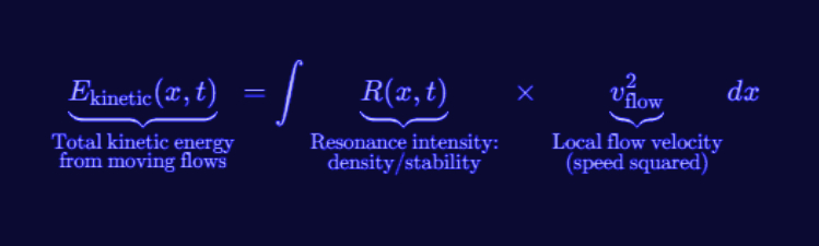
E_kinetic(x, t) = ∫ R(x, t) · v_flow² dx

where:

• R(x, t) is the resonance intensity, representing how dense or stable the flow is at a given point (x, t).
• v_flow is the local flow velocity, showing how fast that portion of the flowfield is moving.
• The integral sums these contributions across the relevant region of space, reflecting that kinetic energy is a global property of the flow rather than something contained in a single particle.

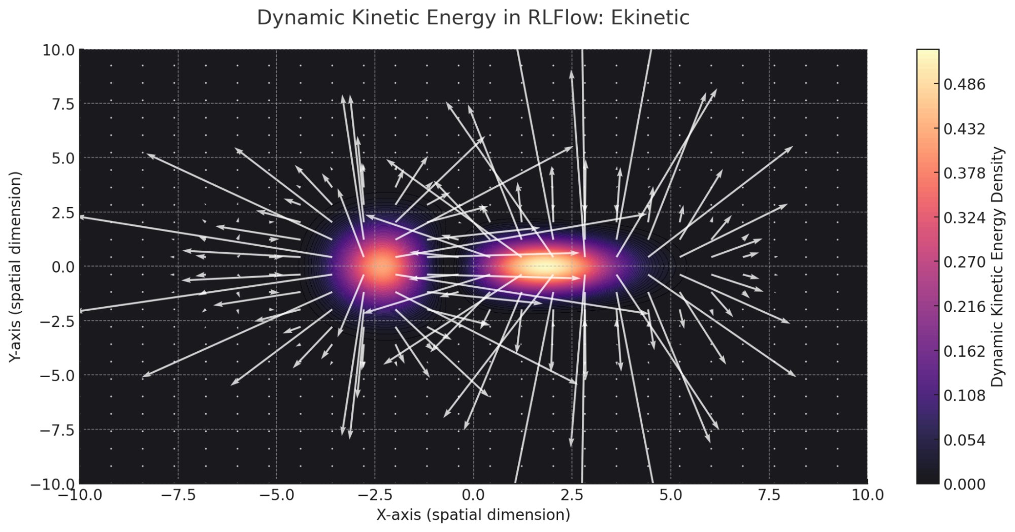
This visualization represents Dynamic Kinetic Energy in RLFlow, showcasing the interplay between resonance intensity and flow dynamics. The color map illustrates the kinetic energy density, while the vectors highlight the energy gradients driving motion within the flowfield.

Particles and Kinetic Energy as Emergent Phenomena

By integrating R(x, t) · v_flow², RLFlow highlights that energy doesn’t belong to isolated objects. Instead, it arises wherever intense, fast-moving flows exist. In many cases, these flows clump into stable patterns that look and act like classical particles—and at large scales, those patterns recover the usual equation ½ m_eff v_eff².

But the key difference is that m_eff and v_eff are effective values derived from the flow’s resonance and movement. In a regime where patterns become clearly “particle-like,” RLFlow mirrors the classical formula as a special case of a deeper, more fluid foundation.

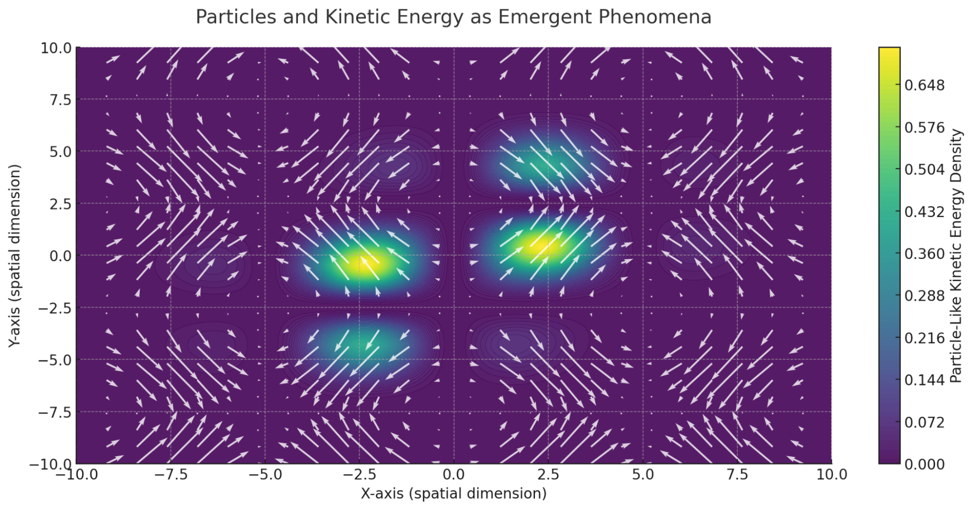
This visualization illustrates Particles and Kinetic Energy as Emergent Phenomena, showing how stable, fast-moving flows clump into patterns resembling classical particles. The color map highlights the kinetic energy density of these particle-like regions, while the vectors depict the dynamic convergence of flows contributing to their stability.

Local Energy Density: A Continuum Perspective

Moving Beyond ½ m v²

In classical physics, kinetic energy is usually a straightforward calculation:

E_k = ½ m v²

However, in a flow-based picture, mass m and velocity v aren’t fundamental inputs. They arise as effective values from the resonance and movement of the flow. To handle this more continuous perspective, RLFlow adopts an approach similar to fluid dynamics:

KE_density = ½ ρ u²,

where ρ is the local “density” (or resonance intensity) of the flow, and u is the local flow speed.

In RLFlow terms:

• ρ ≡ R(x, t), the resonance intensity (how concentrated or stable the flow is).
• u ≡ v_flow, the local speed of the flow pattern at each point.

By integrating this kinetic energy density over the relevant region of space, we obtain the total kinetic energy for that portion of the flowfield:

E_kinetic(x, t) = ∫ R(x, t) · v_flow² dx

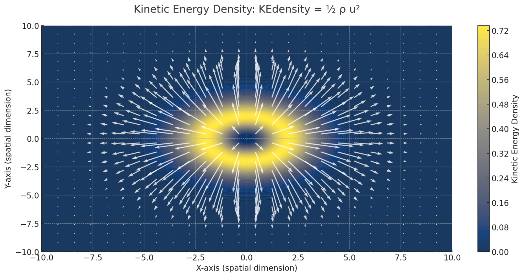
This visualization represents Kinetic Energy Density, where ρ is the resonance intensity and u is the local flow speed. The color map shows how kinetic energy is distributed across the flowfield, while the vectors depict the local flow speed and direction at each point.

A Bridge Between Classical and Emergent Views

Recovering the Familiar Formula

When a region of the flowfield is sufficiently stable—behaving much like a classical object—we can define:

• An effective mass, m_eff, from the integrated resonance intensity.
• An effective velocity, v_eff, from how quickly the peak resonance migrates through space.

At macroscopic scales, these effective values recover the classical kinetic energy form:

KE ≈ ½ m_eff v_eff²

In this way, RLFlow doesn’t discard the traditional approach—it encompasses it as a special case, valid whenever flow patterns act like solid, localized particles.

Connecting to the Quantum World

Unlike pure classical physics, quantum mechanics reveals that particles often behave more like waves spread out in fields. RLFlow’s notion of “mass” and “velocity” as emergent from resonant flows fits more naturally with quantum insights:

• Particles aren’t fundamental; they’re stable wave-like structures.
• Kinetic energy isn’t “owned” by a point-like mass but arises from how the flow (or wavefunction) is distributed and how quickly it evolves in time.

In this sense, RLFlow helps bridge the gap between classical particles and quantum fields by treating both as manifestations of an underlying flowfield—one that can be either well-localized (classical object) or more diffuse (quantum-like).

Metaphor: The River of Resonance

To visualize these ideas, picture a river:

• Rapids and Calm Pools: Where the current is strong and stable, you get a higher resonance intensity R(x, t). Where it’s calm or diffuse, the resonance is lower.
• Local Speed: Different parts of the river can move at different speeds, representing v_flow.
• Energy from the Whole: The river’s total kinetic energy arises from integrating all these local velocities and intensities—just like RLFlow integrates resonance and velocity across a flowfield.

In classical thinking, you might isolate a chunk of water and measure its mass and velocity. In RLFlow, you see the energy as a property of the entire flowing system—fast currents, intense whirlpools, and the interplay between them.

Putting It All Together

1. Mass as Emergent:

   Instead of being a fixed property, mass reflects how stable and tightly bound a resonance pattern is. A more stable pattern behaves more “massive,” resisting changes in motion.

2. Velocity as Flow Dynamics:

   Velocity isn’t an object racing through space but a stable pattern drifting within a larger river of energy. How quickly that pattern moves is its effective velocity.

3. Kinetic Energy as a Derived Quantity:

   By integrating resonance intensity (R) times the square of flow speed (v_flow²), RLFlow captures the total kinetic energy in the system. Classical formulas reappear as a limiting case when flows act like discrete particles.

4. A Unified View:

   This reinterpretation unites classical and quantum perspectives. It shows how an everyday idea like kinetic energy can extend naturally into a field-based description, linking Newtonian mechanics and wave-like quantum phenomena in one flow-based framework.

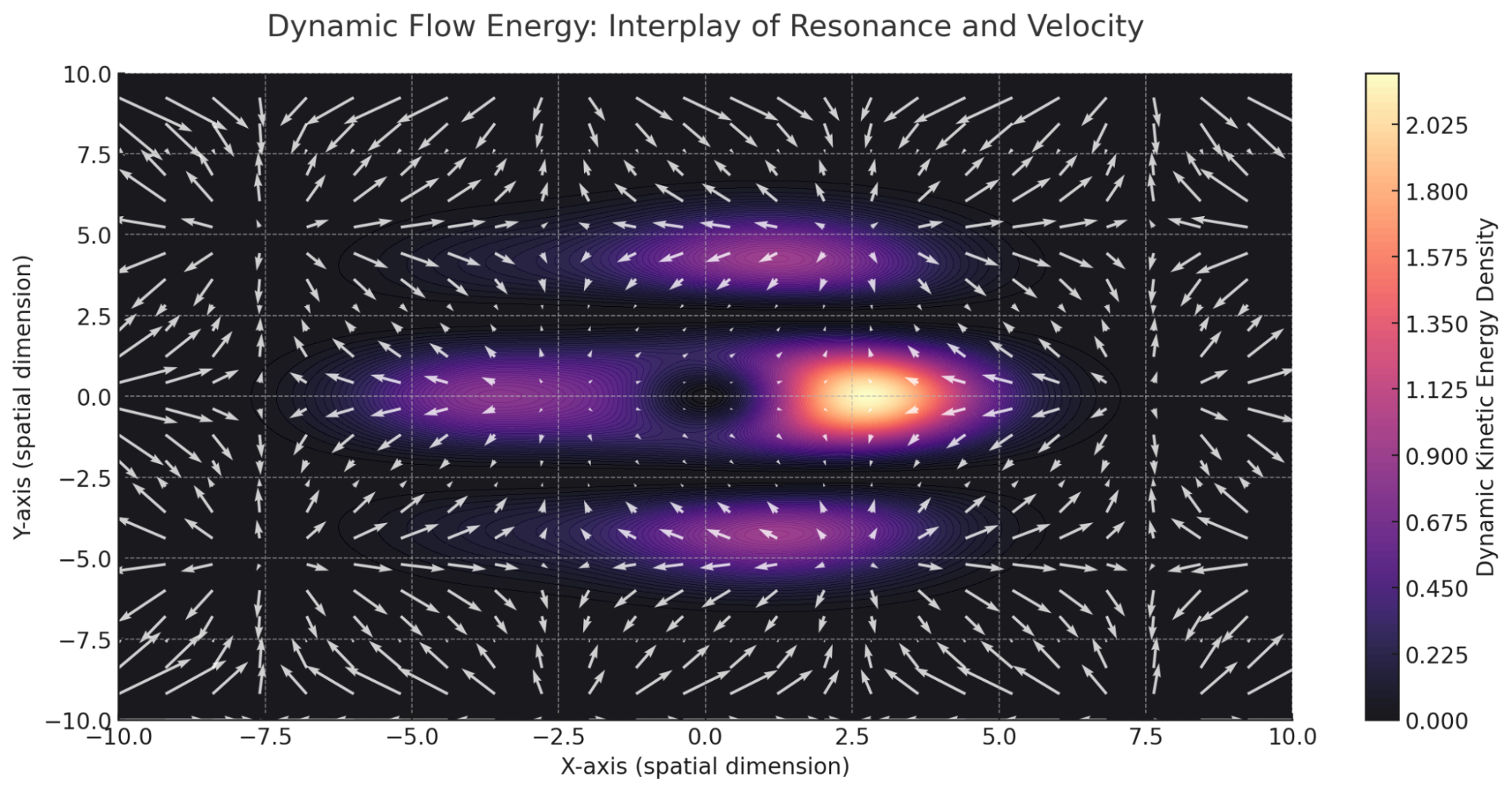
This visualization depicts Dynamic Flow Energy, showcasing the interplay between resonance intensity and local velocity. The color map highlights areas of high kinetic energy density, while the vectors illustrate the dynamic interaction of flows, emphasizing their complexity and movement.

Kinetic vs. Resonance Energy

Key Differences

• Type of Energy Described:
  • Kinetic Energy: Focuses on motion—how fast parts of the flow are moving and how “dense” or “intense” the flow is. Summation (integration) of local kinetic energies across the entire flowfield.
  • Resonance Energy: Focuses on the intrinsic energy of a stable flow pattern—akin to the “rest energy” concept in relativity. A single expression that describes energy inherent in stability.
• When Each Equation Applies:
  • Kinetic Energy Equation: Use this to understand how movement of flows contributes to overall energy (e.g., swirling currents).
  • Resonance Energy Equation: Use this to describe the baseline or rest-like energy inherent in stable flow patterns.

Putting It All Together

• Kinetic (Motion) Energy: Think of a rushing river. Each small portion of water has some speed, contributing to the river’s overall kinetic energy. In RLFlow, this is ∫ R · v_flow² dx.
• Resonance (Rest) Energy: Think of how, in Einstein’s view, mass is “congealed energy.” In RLFlow, a stable, organized flow possesses intrinsic energy by virtue of its resonance, given by E_kinetic = R · C².

Ultimately, both equations highlight two faces of energy in RLFlow: how flows move (kinetic) and how flows simply are (resonance).

Conclusion

We explored how RLFlow redefines mass and velocity as emergent properties of a continuous flowfield. Then, we see how that perspective transforms the concept of kinetic energy, making it a natural outgrowth of resonance and flow dynamics rather than a fixed quantity residing in individual particles.

This fluid approach doesn’t just reframe existing equations—it illuminates a broader, more intuitive understanding of reality. By showing that stable resonances can mimic classical particles, RLFlow allows us to recover the usual ½ m v² formula under certain conditions, yet also broadens our view to include the continuous, interconnected nature of the universe.

Kinetic energy thus becomes part of a grand, flowing fabric, where everything from gentle ripples to roaring rapids contributes to the dynamic dance we call physical reality.

What Each Part Means

E_kinetic(x, t) (Total Flow Kinetic Energy)

This is the overall kinetic energy of the flow in a given region. Instead of belonging to a single “object,” it’s spread out through space, adding up contributions from every point in the flowfield.

R(x, t) (Resonance Intensity)

Think of R as how “dense” or “stable” a particular region of the flow is. High R means the flow pattern is more tightly organized or concentrated—akin to a whirlpool that’s strongly spinning in one spot.

• In classical physics, we’d say “mass.” Here, it’s not a built-in trait but an emergent property reflecting how stable the flow patterns are.

v_flow² (Local Flow Velocity Squared)

This tells us how fast that segment of the flow is moving. Squaring the velocity is familiar from the classical ½ mv² form, capturing the idea that faster-moving flows contribute more heavily to the total kinetic energy.

• In RLFlow, velocity describes how quickly a resonant flow pattern shifts through the surrounding field—not just an “object” traveling in empty space.

∫ … dx (Summation Over Space)

The integral sign indicates we’re adding up these contributions (resonance × velocity-squared) across every point x in the region we care about.

• If you imagine scanning through a river, you’d measure at each little slice how dense the whirlpool is and how fast the current flows, then sum up all those tiny slices to get the total kinetic energy.